Section7.2Comportamiento cualitativo de las soluciones a las EDO
Preguntas Motivadoras
¿Qué es un campo de pendientes?
¿Cómo podemos usar un campo de pendientes para obtener información cualitativa sobre las soluciones de una ecuación diferencial?
¿Cuáles son las soluciones de equilibrio estables e inestables de una ecuación diferencial autónoma?
En trabajos anteriores, hemos usado la línea tangente al gráfico de una función \(f\) en un punto \(a\) para aproximar los valores de \(f\) cerca de \(a\text{.}\) La utilidad de esta aproximación es que necesitamos saber muy poco sobre la función; armados solo con el valor \(f(a)\) y la derivada \(f'(a)\text{,}\) podemos encontrar la ecuación de la línea tangente y la aproximación
Recuerda que una ecuación diferencial de primer orden nos da información sobre la derivada de una función desconocida. Dado que la derivada en un punto nos dice la pendiente de la línea tangente en este punto, una ecuación diferencial nos da información crucial sobre las líneas tangentes al gráfico de una solución. Usaremos esta información sobre las líneas tangentes para crear un campo de pendientes para la ecuación diferencial, lo que nos permite esbozar soluciones a problemas de valor inicial. Nuestro objetivo será entender las soluciones cualitativamente. Es decir, nos gustaría entender la naturaleza básica de las soluciones, como su comportamiento a largo plazo, sin determinar precisamente el valor de una solución en un punto particular.
Usa la ecuación diferencial para encontrar la pendiente de la línea tangente a la solución \(y(t)\) en \(t=0\text{.}\) Luego usa el valor inicial para encontrar la ecuación de la línea tangente en \(t=0\text{.}\) Dibuja esta línea tangente sobre el intervalo \(-0.25 \leq t \leq 0.25\) en los ejes proporcionados en Figure 7.2.1.
Figure7.2.1.Cuadrícula para trazar líneas tangentes parciales.
También se muestran en Figure 7.2.1 las líneas tangentes a la solución \(y(t)\) en los puntos \(t=1, 2\text{,}\) y \(3\) (veremos cómo encontrarlas más adelante). Usa el gráfico para medir la pendiente de cada línea tangente y verifica que cada una coincide con el valor especificado por la ecuación diferencial.
Usando estas líneas tangentes como guía, dibuja un gráfico de la solución \(y(t)\) sobre el intervalo \(0\leq t\leq 3\) de manera que las líneas sean tangentes al gráfico de \(y(t)\text{.}\)
Usa el Teorema Fundamental del Cálculo para encontrar \(y(t)\text{,}\) la solución a este problema de valor inicial.
Grafica la solución que encontraste en (d) en los ejes proporcionados, y compárala con el dibujo que hiciste usando las líneas tangentes.
Subsection7.2.1Campos de pendientes
Actividad de Previsualización 7.2.1 muestra que podemos esbozar la solución a un problema de valor inicial si conocemos una colección apropiada de líneas tangentes. Podemos usar la ecuación diferencial para encontrar la pendiente de la línea tangente en cualquier punto de interés, y por lo tanto trazar dicha colección.
Sigamos mirando la ecuación diferencial \(\frac{dy}{dt} = t-2\text{.}\) Si \(t=0\text{,}\) esta ecuación dice que \(dy/dt = 0-2=-2\text{.}\) Nota que este valor se mantiene independientemente del valor de \(y\text{.}\) Por lo tanto, esbozaremos líneas tangentes para varios valores de \(y\) y \(t=0\) con una pendiente de \(-2\text{,}\) como se muestra en Figura 7.2.2.
Figure7.2.2.Líneas tangentes en puntos con \(t=0\text{.}\)
Figure7.2.3.Agregando líneas tangentes en puntos con \(t=1\text{.}\)
Sigamos de la misma manera: si \(t=1\text{,}\) la ecuación diferencial nos dice que \(dy/dt = 1-2=-1\text{,}\) y esto se mantiene independientemente del valor de \(y\text{.}\) Ahora esbozamos líneas tangentes para varios valores de \(y\) y \(t=1\) con una pendiente de \(-1\) en Figura 7.2.3.
De manera similar, vemos que cuando \(t=2\text{,}\)\(dy/dt = 0\) y cuando \(t=3\text{,}\)\(dy/dt=1\text{.}\) Por lo tanto, podemos agregar a nuestra creciente colección de gráficos de líneas tangentes para lograr Figura 7.2.4.
Figure7.2.4.Agregando líneas tangentes en puntos con \(t=2\) y \(t=3\text{.}\)
Figure7.2.5.Un campo de pendientes completo.
En Figura 7.2.4, comenzamos a ver emerger las soluciones a la ecuación diferencial. Para mayor claridad, agregamos más líneas tangentes para proporcionar la imagen más completa que se muestra a la derecha en Figura 7.2.5.
Figura 7.2.5 se llama un campo de pendientes para la ecuación diferencial. Nos permite esbozar soluciones tal como lo hicimos en la actividad de previsualización. Podemos comenzar con el valor inicial \(y(0) = 1\) y empezar a esbozar la solución siguiendo la línea tangente. Siempre que la solución pase por un punto en el que se haya dibujado una línea tangente, esa línea es tangente a la solución. Este principio nos lleva a la secuencia de imágenes en Figura 7.2.6.
Figure7.2.6.Una secuencia de imágenes que muestra cómo esbozar la solución del PVI que satisface \(y(0)=1\text{.}\)
De hecho, podemos dibujar soluciones para cualquier valor inicial. Figura 7.2.7 muestra soluciones para varios valores iniciales diferentes para \(y(0)\text{.}\)
Figure7.2.7.Diferentes soluciones a \(\frac{dy}{dt} = t-2\) que corresponden a diferentes valores iniciales.
Así como lo hicimos para la ecuación \(\frac{dy}{dt} = t-2\text{,}\) podemos construir un campo de pendientes para cualquier ecuación diferencial de interés. El campo de pendientes nos proporciona información visual sobre cómo esperamos que se comporten las soluciones de la ecuación diferencial.
Haz un gráfico de \(\frac{dy}{dt}\) versus \(y\) en los ejes proporcionados en Figura 7.2.8. Mirando el gráfico, ¿para qué valores de \(y\) aumenta \(y\) y para qué valores de \(y\) disminuye \(y\text{?}\)
Figure7.2.8.Ejes para graficar \(\frac{dy}{dt}\) versus \(y\text{.}\)
Figure7.2.9.Ejes para graficar el campo de pendientes para \(\frac{dy}{dt} = -\frac 12( y - 4)\text{.}\)
A continuación, dibuja el campo de pendientes para esta ecuación diferencial en los ejes proporcionados en Figura 7.2.9.
Usa tu trabajo en (b) para dibujar (en los mismos ejes en Figura 7.2.9.) soluciones que satisfacen \(y(0) = 0\text{,}\)\(y(0) = 2\text{,}\)\(y(0) = 4\) y \(y(0) = 6\text{.}\)
Verifica que \(y(t) = 4 + 2e^{-t/2}\) es una solución a la ecuación diferencial dada con el valor inicial \(y(0) = 6\text{.}\) Compara su gráfico con el que dibujaste en (c).
¿Qué es especial acerca de la solución donde \(y(0) = 4\text{?}\)
Subsection7.2.2Soluciones de equilibrio y estabilidad
Como nuestro trabajo en Actividad 7.2.2 demuestra, las ecuaciones autónomas de primer orden pueden tener soluciones que son constantes. Estas son simples de detectar inspeccionando la ecuación diferencial \(dy/dt = f(y)\text{:}\) las soluciones constantes necesariamente tienen una derivada cero, así que \(dy/dt = 0 = f(y)\text{.}\)
Por ejemplo, en Actividad 7.2.2, consideramos la ecuación \(\frac{dy}{dt} = f(y)=-\frac12(y-4)\text{.}\) Las soluciones constantes se encuentran estableciendo \(f(y) = -\frac12(y-4) = 0\text{,}\) lo que inmediatamente vemos que implica que \(y = 4\text{.}\)
Valores de \(y\) para los cuales \(f(y) = 0\) en una ecuación diferencial autónoma \(\frac{dy}{dt} = f(y)\) se llaman soluciones de equilibrio de la ecuación diferencial.
Haz un gráfico de \(\frac{dy}{dt}\) versus \(y\) en los ejes proporcionados en Figura 7.2.10. Mirando el gráfico, ¿para qué valores de \(y\) aumenta \(y\) y para qué valores de \(y\) disminuye \(y\text{?}\)
Figure7.2.10.Ejes para graficar \(dy/dt\) vs \(y\) para \(\frac{dy}{dt} = -\frac 12 y(y-4)\text{.}\)
Figure7.2.11.Ejes para graficar el campo de pendientes para \(\frac{dy}{dt} = -\frac 12 y(y-4)\text{.}\)
Identifica cualquier solución de equilibrio de la ecuación diferencial dada.
Ahora dibuja el campo de pendientes para la ecuación diferencial dada en los ejes proporcionados en Figura 7.2.11.
Dibuja las soluciones a la ecuación diferencial dada que corresponden a valores iniciales \(y(0)=-1, 0, 1, \ldots, 5\text{.}\)
Una solución de equilibrio \(\overline{y}\) se llama estable si las soluciones cercanas convergen a \(\overline{y}\text{.}\) Esto significa que si la condición inicial varía ligeramente de \(\overline{y}\text{,}\) entonces \(\lim_{t\to\infty}y(t) = \overline{y}\text{.}\) Por el contrario, una solución de equilibrio \(\overline{y}\) se llama inestable si las soluciones cercanas se alejan de \(\overline{y}\text{.}\) Usando tu trabajo anterior, clasifica las soluciones de equilibrio que encontraste en (b) como estables o inestables.
Supón que \(y(t)\) describe la población de una especie de organismos vivos y que el valor inicial \(y(0)\) es positivo. ¿Qué puedes decir sobre el destino final de esta población?
Ahora considera una ecuación diferencial autónoma general de la forma \(dy/dt = f(y)\text{.}\) Recuerda que una solución de equilibrio \(\overline{y}\) satisface \(f(\overline{y}) = 0\text{.}\) Si graficamos \(dy/dt = f(y)\) como una función de \(y\text{,}\) ¿para cuál de las ecuaciones diferenciales representadas en Figura 7.2.12 y Figura 7.2.13 es \(\overline{y}\) un equilibrio estable y para cuál es \(\overline{y}\) inestable? ¿Por qué?
Figure7.2.12.Gráfico de \(\frac{dy}{dt}\) como una función de \(y\text{.}\)
Figure7.2.13.Gráfico de \(\frac{dy}{dt}\) como una función diferente de \(y\text{.}\)
Subsection7.2.3Resumen
Un campo de pendientes es un gráfico creado trazando las líneas tangentes de muchas soluciones diferentes a una ecuación diferencial.
Una vez que tenemos un campo de pendientes, podemos esbozar el gráfico de soluciones dibujando una curva que siempre sea tangente a las líneas en el campo de pendientes.
Las ecuaciones diferenciales autónomas a veces tienen soluciones constantes que llamamos soluciones de equilibrio. Estas pueden clasificarse como estables o inestables, dependiendo del comportamiento de las soluciones cercanas.
Exercises7.2.4Exercises
1.Graphing equilibrium solutions.
Consider the direction field below for a differential equation. Use the graph to find the equilibrium solutions.
Answer (separate by commas):\(y =\)
Note:You can click on the graph to enlarge the image.
2.Sketching solution curves.
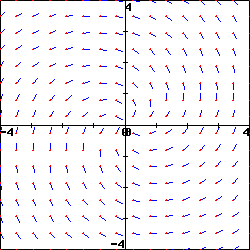
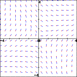
Consider the two slope fields shown, in figures 1 and 2 below.
figure 1
figure 2
On a print-out of these slope fields, sketch for each three solution curves to the differential equations that generated them. Then complete the following statements:
For the slope field in figure 1, a solution passing through the point (4,-3) has a
positive
negative
zero
undefined
slope.
For the slope field in figure 1, a solution passing through the point (-2,-3) has a
positive
negative
zero
undefined
slope.
For the slope field in figure 2, a solution passing through the point (2,-1) has a
positive
negative
zero
undefined
slope.
For the slope field in figure 2, a solution passing through the point (0,3) has a
positive
negative
zero
undefined
slope.
3.Matching equations with direction fields.
Match the following equations with their direction field. Clicking on each picture will give you an enlarged view. While you can probably solve this problem by guessing, it is useful to try to predict characteristics of the direction field and then match them to the picture.
Here are some handy characteristics to start with -- you will develop more as you practice.
Set \(y\) equal to zero and look at how the derivative behaves along the \(x\)-axis.
Do the same for the \(y\)-axis by setting \(x\) equal to \(0\)
Consider the curve in the plane defined by setting \(y'=0\) -- this should correspond to the points in the picture where the slope is zero.
Setting \(y'\) equal to a constant other than zero gives the curve of points where the slope is that constant. These are called isoclines, and can be used to construct the direction field picture by hand.
Given the differential equation \(x'(t) = - x^4 - 9x^3 - 19x^2 + 9x + 20\text{.}\)
List the constant (or equilibrium) solutions to this differential equation in increasing order and indicate whether or not these equilibria are stable, semi-stable, or unstable. (It helps to sketch the graph. 1
Sketch the solutions whose initial values are \(y(0)= -4, -3, \ldots, 4\text{.}\)
What do your sketches suggest is the solution whose initial value is \(y(0) = -1\text{?}\) Verify that this is indeed the solution to this initial value problem.
By considering the differential equation and the graphs you have sketched, what is the relationship between \(t\) and \(y\) at a point where a solution has a local minimum?
6.
Consider the situation from problem 2 of Section 7.1: Suppose that the population of a particular species is described by the function \(P(t)\text{,}\) where \(P\) is expressed in millions. Suppose further that the population’s rate of change is governed by the differential equation
Sketch a slope field for this differential equation. You do not have enough information to determine the actual slopes, but you should have enough information to determine where slopes are positive, negative, zero, large, or small, and hence determine the qualitative behavior of solutions.
Sketch some solutions to this differential equation when the initial population \(P(0) \gt 0\text{.}\)
Identify any equilibrium solutions to the differential equation and classify them as stable or unstable.
If \(P(0) \gt 1\text{,}\) what is the eventual fate of the species? if \(P(0) \lt 1\text{?}\)
Remember that we referred to this model for population growth as “growth with a threshold.” Explain why this characterization makes sense by considering solutions whose inital value is close to 1.
7.
The population of a species of fish in a lake is \(P(t)\) where \(P\) is measured in thousands of fish and \(t\) is measured in months. The growth of the population is described by the differential equation
Sketch a graph of \(f(P) = P(6-P)\) and use it to determine the equilibrium solutions and whether they are stable or unstable. Write a complete sentence that describes the long-term behavior of the fish population.
Suppose now that the owners of the lake allow fishers to remove 1000 fish from the lake every month (remember that \(P(t)\) is measured in thousands of fish). Modify the differential equation to take this into account. Sketch the new graph of \(dP/dt\) versus \(P\text{.}\) Determine the new equilibrium solutions and decide whether they are stable or unstable.
Given the situation in part (b), give a description of the long-term behavior of the fish population.
Suppose that fishermen remove \(h\) thousand fish per month. How is the differential equation modified?
What is the largest number of fish that can be removed per month without eliminating the fish population? If fish are removed at this maximum rate, what is the eventual population of fish?
8.
Let \(y(t)\) be the number of thousands of mice that live on a farm; assume time \(t\) is measured in years. 2
This problem is based on an ecological analysis presented in a research paper by C.S. Hollings: The Components of Predation as Revealed by a Study of Small Mammal Predation of the European Pine Sawfly, Canadian Entomology91: 283-320.
The population of the mice grows at a yearly rate that is twenty times the number of mice. Express this as a differential equation.
At some point, the farmer brings \(C\) cats to the farm. The number of mice that the cats can eat in a year is
thousand mice per year. Explain how this modifies the differential equation that you found in part a).
Sketch a graph of the function \(M(y)\) for a single cat \(C=1\) and explain its features by looking, for instance, at the behavior of \(M(y)\) when \(y\) is small and when \(y\) is large.
Suppose that \(C=1\text{.}\) Find the equilibrium solutions and determine whether they are stable or unstable. Use this to explain the long-term behavior of the mice population depending on the initial population of the mice.
Suppose that \(C=60\text{.}\) Find the equilibrium solutions and determine whether they are stable or unstable. Use this to explain the long-term behavior of the mice population depending on the initial population of the mice.
What is the smallest number of cats you would need to keep the mice population from growing arbitrarily large?